Never Tell Me The Odds

Author

Affiliation

Keller Liptrap

Allegheny College

Abstract

This project developed a tool that uses data from the past five NBA seasons and machine learning models to predict the outcomes of NBA games. This tool leverages the growing access to and interest in advanced sports analytics. The tool named “Never Tell Me the Odds” provides a user-friendly dashboard to display predictions of NBA games for sports fanatics all around the world. The tool uses the nba_api to gather historical data, which is used and processed by machine learning algorithms to generate predictions. The backend of the tool handles all of the processing and training of the data, while the front end is a straightforward dashboard to show each of the predicted winners made by the models. The various machine learning algorithms, including linear regression, random forest, and support vector machines, were compared to find the most effective for NBA game prediction. Several experiments evaluate the tool’s performance to determine what influences the accuracy of predicting real-world NBA games. The result of the project indicates that there is potential for machine learning to predict NBA game outcomes. The tool and project offer insights for fans, analysts, and sports bettors. With this being said, there is an acknowledgment of the limitation of the machine learning models, such as player injuries or trades, as well as ethical considerations when it comes to sports betting.

Introduction

      The National Basketball Association is one of the most popular sports leagues worldwide. Millions of fans tune in for the fast-paced play of today’s game as well as the teams and players that they are diehard fans of. With the rise of advanced analytics and predictive algorithms such as machine learning, predicting NBA games has become a hot topic for sports enthusiasts, analysts, and sports bettors. This project developed a tool that uses historical data and statistical models to predict game outcomes. Using the large fanbase of the NBA and predictive analytics, this tool is an innovation for fans, teams, and professionals.

Motivation

      In the United States alone, there were an estimated 95.5 million sports viewers in 2023, a number projected to rise by 30 million within the next four years, reflecting the ever-growing love for sports across the nation [6]. But underneath the surface, sports is a data-driven system. Data influences how teams strategize, shapes how fans engage with their favorite teams, and is the driver of the ever-growing sports betting industry. Among all sports, basketball stands out as being popular across the globe, with leagues from China and Serbia. At the forefront of this global appeal is the NBA, the largest league in the world, located in the United States. During the most recent NBA season in 2023 and 2024, there was an average of 1.5 million viewers for a regular season game. The number of viewers would rise based on in-season tournament games or when playoffs came at the end of the season, especially during the NBA championship, where average viewers per game would jump to about 11 million [29].

      With the growing global popularity of basketball and the increasingly data-driven nature of modern sports, I developed a tool that predicts the outcome of NBA games. This tool used NBA box score data such as points, rebounds, and three-point percentages, along with advanced analytics like player efficiency rating and plus-minus score. The analytics come from the past five years of the NBA. The data collected from previous teams’ games powers machine learning algorithms, enabling more accurate predictions compared to traditional win-loss analysis. This tool benefits all sports fans, from casual viewers to NBA enthusiasts, offering insights into game dynamics and sports betting opportunities. Predictions and game updates are provided on a user-friendly dashboard that updates daily. With the growing global interest in basketball analytics, this tool provides valuable insights into how fans engage with the game and make informed predictions.

      The NBA extends farther than the court and television with a large and influential social media presence. With 210 million followers on social media, the NBA is number one and has more followers than the NFL, NHL, MLB, and MLS combined. The growing influence of social media shows no signs of stopping. Between 2018 and 2021, the NBA, across all media platforms, gained roughly 60 million followers. Within the NBA, there are 30 teams across the United States and Canada. Each team has a unique fanbase from all across the globe. These teams have an average of 17 million followers across social media. Some fan-favorite teams, such as the Los Angeles Lakers and the Golden State Warriors, gain mass followings from people across the world. The Lakers, who have the highest following on social media and fan base on social media, make up about 11 % of all teams, and right behind them are the Warriors. Teams like this are just half the story when talking about the popularity of the NBA. Players on every team have die-hard fans who follow them from team to team, and their fan bases are continuing to grow and influence basketball fans. There is no better example of this than LeBron James. LeBron has well over 200 million followers across all media platforms and has generated billions of views on social media platforms for the NBA [5]. The NBA extends far beyond just basketball fans, attracting a diverse audience across the world. Among all sports, the NBA is the most diverse, with Hispanic and African American viewers. Not only is the NBA diverse in viewers’ ethnicity, but it is also diverse in the ages of those watching the NBA. The average viewer and attendee of NBA games are in their mid-30s, with 42 % of people between the ages of 45 and 64 considering themselves fans of the NBA. The highest number of fans comes in the 18-34 age bracket, where 62 % of people asked in this age range say they are fans of the NBA [5]. Television and attending games are not the only ways fans interact with the game of basketball. There has been a rise in fantasy sports, where individuals draft players for their team and go head-to-head with their friends. According to ESPN, there are well over 2 million fans who played fantasy basketball during last year’s NBA season, marking a 5% increase from the year before [22]. Aside from the growing popularity of basketball and the NBA, there has been a rise in the use of analytics that has revolutionized how fans and analysts approach and interact with sports.

      Advanced metrics are just one of the ways that the NBA has incorporated advanced data into player stats. Efficiency Rating (PER), True Shooting Percentage (TS%), and Box Plus-Minus (BPM) are just a few of these advanced statistics that offer a more profound analysis of how teams and players are doing that goes beyond the traditional stats such as points, rebounds, and assists. This allows fans to take a deep dive into stats that are contributing to their team winning and losing and create their own opinions as to what their team should do, which can lead to more engagement from fans. Advanced analytics can also serve a purpose that is personalized to NBA players. With the use of machine learning, predictive models can take into account players’ workloads, fatigue, and biomechanics. This data can be used to prevent injury while limiting players on and off the court and can help develop workout plans for these high-level athletes. Although this benefits the players directly, it also helps keep fan engagement. This allows players to be on the court for more games and contribute to the success of the team. In return, this keeps fans engaged and watching games when they might not have if their favorite player is out for the game. Another way fan engagement has evolved is due to the shift towards personalized and immersive experiences that enhance engagement. Mentions earlier that social media is a platform that is used by the NBA and all its teams to promote and connect with their fans. The NBA and teams can leverage the data from these platforms to get an understanding of fan preferences and emotional responses. This can allow organizations to strategize events or posts that can boost fans’ mood and engagement. Machine learning can also be used to anticipate fan preferences and suggest the timing and type of promotions or content. In addition to this, personalized apps or website content and offers can be offered to fans based on interests to deepen fan loyalty and interaction [21].

      In recent years, there has been a boom in the sports betting industry. Sports betting sites like FanDuel and DraftKings garner billions of dollars per year from fans betting on all aspects of sports. On sports betting sites, there are a variety of different bets that an individual can make. The first category of bets that can be made is on teams. Individuals can bet on the spread of the game, whether a specific team is going to win or lose by a certain amount. In a single game, individuals can also bet on the total, which in the NBA is the total number of points scored from both teams. This bet can be placed on either over or under that point value designated by the sports betting site. Finally, in this section of sports betting, you can bet on the money line, which is essentially choosing who you think is going to win the game. The second category of betting in the NBA is betting on player lines, such as how many points they will score or how many rebounds will be scored. These types of bets can be done by quarter, by half, and/or by the full game depending on what the sports betting site allows. There are also special one-off categories, such as who will score the first point in the game. The big appeal of sports betting comes with parlays, which involve taking more than one bet at a time to increase the odds because it is more unlikely that all of the bets will happen, and in return, the user will win more money.

Current State of the Art

      Predicting NBA game outcomes combines the excitement and popularity of the game and the power of advanced stats and analytics. The NBA provides a large amount of data and stats that can be used for data analysis for predicting the winner of games. Fans, analysts, and sports bettors use tools such as ESPN BPI, which provides rankings for teams based on the average stats in a category using advanced stats. With this being said, predictive models and tools for the NBA have their drawbacks. Tools may not account for players or last-minute lineup changes. These tools are also designed by more experts. Without the knowledge of the tools, users may not understand how to work or use the tools. This can create a less user-friendly experience. This creates an opportunity for a tool for NBA prediction that is user-friendly and easy to understand that can bring fans closer to the game.

      There are a couple of traditional statistical models that are used to create predictions of games. First is the use of Elo ratings. Elo rating systems are used in a variety of sports today but were originally used to predict chess games. It is used in the NBA today to rate teams or players based on match-by-match comparisons from team to team or player to player. Prediction is based on rating differences between the two teams that are playing or the two players that are head to head. The Elo system has adjusted ratings after each game based on wins and losses. There are several key principles in the Elo system. First is that the higher-rated teams are more likely to be predicted to win, and the higher the margin of rating, the higher the probability a team is to win. Second, teams that are lower-rated that get wins over higher-rated teams get a boost in rating changes after a game. Finally, the Elo system is zero-sum. This means that points that are gained by winners and losers are equal. This allows for consistency across all games [17].

      Second is predicting point differentials in the NBA to predict the outcomes of games. Point differential is simply how many points a team scores versus the number of points that are scored on them. To determine point differential prediction, previous season data is used to determine a team’s ability and home advantages for teams. This also has its limitations, as it does not account for players who have missed games, currently injured players, or players that may have signed or have been traded to a new team. These factors can contribute to a change in point differential if they are not calculated in the model [13].

      Machine learning has transformed how we can predict outcomes in sports. It offers tools and libraries that are powerful and help uncover patterns in data. Machine learning models differ from traditional modeling that has set equations; rather, these models can transform and adapt around the data that is given. The NBA is full of advanced stats, and these models can take into account these variables and find relationships between them to offer a prediction of a winner that otherwise would not be possible given traditional algorithms. There are many machine learning algorithms that can be used to predict the outcome of an NBA game.

      First, linear regression models are the most straightforward of them. In a linear regression model, variables are given such as points, rebounds, and/or assists. Each of these variables may carry a different weight in terms of their importance to winning an NBA game. Using this information, teams are able to compare to one another when facing off, and the team with the higher favored variables will be predicted as the winner. Logistic regression is also used to predict the outcome of NBA games by using a binary outcome such as a win or a loss. For instance, a variable of three-point percentage for a team is assigned a number between 0 and 1; this is then used to calculate how impactful this variable is on the team’s winning or losing [20].

      Random forests is a machine learning algorithm that is a large number of decision trees. Each decision tree has its own prediction based on one variable within it. These predictions are then all taken and averaged together to get an overall prediction. In terms of the NBA, if points, rebounds, and assist stats are given to this model, it will take both teams data for each of those categories and create individual decision trees for the specific teams variables. Based on the prediction within these trees, it will give an overall winner for the game [20].

      Many tools and resources provide data for predictions, as well as many tools that predict the outcomes of NBA games. These tools have been created to help analysts and fans interact with the game in unique ways. Sites such as Official NBA Stat and Basketball Reference provide stats to those looking to predict NBA games. Many projects use these sites and APIs to get their data for their machine learning algorithms. Sports betting sites use predictive modeling to set their bets for a given NBA game. The use of predictive models heavily influences the sports betting market. This is just one example of a large-scale use of machine learning. There are many smaller projects on GitHub predicting various NBA stats from player performance, the most valuable player for a given year, and the outcome of NBA games.

Goals of the Project

      The goal of my tool called Never Tell Me the Odds was to correctly predict the outcomes of NBA games using machine learning. Using data from box scores from previous seasons of the NBA for machine learning algorithms, the tool aimed to correctly predict the outcome of a given day’s NBA games. My tool aimed to give users, who were fans and analysts, a simple and user-friendly resource for predictive NBA analytics. The objective of the tool was to be able to predict the outcomes of NBA games based on the daily schedule of the NBA. The tool read the day’s games and, using the already-trained model, predicted the winner of the game.

      The backend of this tool used historical data from the past 5 NBA seasons. This data was cleaned, sorted, and used when creating the predictive model using machine learning libraries. The model was then used to predict the games. The current day’s games were also pulled from the NBA-API. These teams were used in the model to predict the winner of the matchup. The front end of the tool was a dynamic dashboard that was updated daily so users could look at the predicted outcomes for that day’s NBA games. This provided a friendly user experience, as it was simple and clean to look at and understand. The dashboard showed the home and away teams’ names and displayed their logo. The time that the game was played was also shown in the dashboard for those who might have been sports betting and needed to place their bets. Additionally, the predicted winner of the game was shown in the same row as the games for the day. Finally, there was a confidence level for how accurate the model believed this prediction was. Additional information like confidence gave the user more insight into the predictive capabilities of the tool.

      Overall, this tool provided a resource for fans, analysts, and sports bettors to get a better insight into NBA games. Fans gained more insight into their favorite teams. Analysts could use this information and data to better assess and understand why teams were winning and losing. Sports bettors used the predictions to inform and make better bets based on the winners and losers of the game, as well as the confidence level of the prediction. With the growing trend in data and analytics, this tool made it easier for all to understand how they affected the outcomes of NBA games.

      Many machine learning algorithms, such as linear regression, logistic regression, and random forests, can be used to predict the outcome of NBA games. Each of the possible machine learning algorithms is tested on a set of games. The purpose of this is to determine which of the algorithms has the best percentage of games predicted. The one with the highest will be the central predictive model for this tool. For the data for the predictive models, the NBA-API will be used. This API provides access to a wide variety of data and NBA analytics. Traditional stats like points, rebounds, and assists as well as advanced stats such as player plus-minus will be collected through the API.

Ethical Implications

      As any developer making a tool, there are ethical implications that should be considered when creating a tool that predicts NBA games. There is a growing market of sports bettors that this tool speaks to, which should not be ignored. Tools such as this one that give predictive stats may encourage individuals to gamble their money on games [3]. As the tool is never going to be correct all the time, this can lead to bets that might be risky and result in a loss of money. Making sure users know that gambling is risky regardless of the predictive stats is key. This makes sure those who may have a gambling problem may be enticed to fully trust the tool that it’ll be right, as well as encouraging bets from those individuals.

      There is a large amount of data that is being collected for predictive modeling in this tool. It is important to note that this data may have biases, such as not reflecting player injuries, player trades, and other immeasurable variables that might lead to a team’s stats dipping or taking an unexpected turn. This type of bias would not be reflected in the model due to it solely looking at stats and not outside variables to these stats. It is important to look at and acknowledge that machine learning has limitations. It will correctly predict the outcome in every game, and it is important to stress the importance of the tool’s limitations to its users.

      Overall, it is important to be open and honest with users about the tool. Taking accountability for code that is not up to par or providing a bad prediction is key, as well as the previously mentioned data biases [31]. Owning coding mistakes and expressing what happened and why it happened is important. Giving information on what modeling is used and how it is used can help users understand how the tool is supposed to work rather than users guessing if it is correct. In addition to making it known what the machine learning algorithm is being used for, it is important to let users know what variables are going to be used to make the model that is predicting the games. Finally, acknowledging the tool’s limitations in calculating all variables is important to the users. The key limitation to note is the accuracy of the tool. Running tests and letting users know our findings on the accuracy of the tool is important.

      To address possible ethical implications, I plan to take several steps. The first is creating warnings on the dashboard page. These warnings will inform the user to use the tool for betting at their own risk. This warning will include that the accuracy of the tool might not be 100 % and predict all the games correctly. Much like sports betting apps do, there will be a link and description to get help for those who have a gambling addiction. While running tests for the tool to find which machine learning algorithm is the best, there will be accuracy kept by keeping track of how many games the algorithm predicts correctly. This will be displayed in the ReadMe file with a designated section. Additionally, in this section, details about data biases and the limitations of the tool.

Related Work

    This section is going to review existing research on NBA games. Sports prediction has been an increasing topic in academic research. Studies look at creating statistical models, testing machine learning methods, and identifying important factors that might influence the outcome of an NBA game. In addition to this, researchers have also pointed out the challenges they are faced with when working with predictive algorithms.

Advanced Analytics

    Advanced analytics play a key role in the evaluation of team performance and its players’ performance. There are several metrics, such as Adjusted Plus-Minus and Win Shares, that provide more profound insights into a player’s impact that statistics like points and rebounds may not provide. Research by Vangelis Sarlis and Christos Tjortjis emphasizes that while advanced metrics can show a player’s true impact on a game, such information is not without its limitations. For instance, certain matchups can pose unique challenges. This makes it difficult to rely just on these analytics for predicting NBA game outcomes. This highlights the importance of combining advanced analytics with human judgment to make informed decisions [28]. This balance is relevant in the creation of this tool that uses predictive models and a large amount of data. The data by itself may not capture all the complexities of an NBA game, which may lead to inaccurate predictions.

    The value of data and analytics goes far beyond performance evaluation but can be used for broader insights into sports franchises. For example, the Tampa Bay Lightning uses analytics not just to enhance their team’s performance but also to improve fan experiences and specific marketing strategies. This demonstrates the versatility of today’s data and its potential applications. With this being said, implementing systems comes with some challenges, especially for smaller sports franchises. Smaller franchises may not have the resources to manage large data structures [18]. In contrast, NBA teams benefit from a rapidly growing economy. These teams are better positioned to adopt advanced analytics for both organizational improvement and fan engagement. Predictive tools for NBA games offer opportunities to support targeted promotions by identifying games that would be highly successful. This creates an advantage in fan outreach for NBA franchises.

    The integration of analytics into sports also creates innovation across the league. Having a centralized system such as SportVu, which is used by the NBA, makes sure that all teams have the same access to data regardless of what the size of the franchise is. This creates a level playing field for all teams. In addition to teams, players and whoever they train with can leverage data to improve their craft. Data can be used to optimize training and reduce injury risks. In addition to players and teams, analytics can engage fans, especially those who are interested in contributing to the advancements around the league. Since analytics have become more widespread, the competitive advantage that they offer can diminish. As more teams use these analytics and have dedicated teams interpreting the data, the less and less of an advantage these analytics can have. There is still an issue of smaller franchises not having the resources to have an analytics team in their building and may need to rely on external experts, which can limit the gain from the analytics [21]. This information emphasizes the power of data in sports but also shows the challenges and limitations that come with them. Prediction tools such as this one that are designed to be user-friendly and accessible can help with some of these challenges and limitations. It can help teams, fans, and organizations understand and leverage analytics to improve all aspects of their franchise.

Machine Learning

    In the article titled “Machine Learning Algorithms A Review” by Batta Mahesh, the author discusses the details of machine learning and its various algorithms. Machine learning algorithms can be categorized into supervised and unsupervised learning. Supervised learning uses algorithms like decision trees and support vector machines to classify and predict. Unsupervised learning relies on algorithms like K-clusters to analyze data and find patterns. Additionally, semi-supervised learning combines both of these approaches and is useful for data sets that have some amount of data that is labeled. There is also reinforcement learning, which makes decisions over time through trial and error. This can be useful in robotics and gaming. Finally, deep learning is used when working with large data sets requiring complex pattern recognition and analysis. Each of these methods has its benefits and drawbacks. Supervised learning relies heavily on labeled data, while unsupervised learning can identify patterns but may be difficult to interpret. Overall, Mahesh provides a well-structured discussion by organizing the paper by different learning types and what models are used for each of the learning types [14]. Understanding these categories is important for building predictive tools, as selecting the right type of machine learning depends on the data available and the specific goals of the model.

    Predictions have become an increasingly popular and important topic in machine learning research. One study investigates learning-based prediction systems by analyzing their accuracy, ease of interpretation, and usability. The study examines four machine learning algorithms: Artificial Neural Networks (ANNs), Case-Based Reasoning (CBR), Rule Induction (RI), and Least Squares Regression (LSR). ANN was found to be the most accurate, but its performance changed depending on the dataset used [16]. With this being said, ANN can be complex to set up and interpret, which can make it a potential drawback for prediction models. CBR and LSR were moderately accurate. CBR performed better when users could adjust it to specific cases. LSR struggled with outliers, which had an impact on prediction accuracy. RI was the least accurate; it only improved when fewer variables were used. This study provides a unique perspective by considering not just accuracy but also usability and interpretability. These factors are often overlooked when evaluating algorithms. One limitation of this study is the use of a small dataset. Using the findings of this study and applying them to a large dataset for NBA game prediction could affect and change the results. The study also highlights the importance of efficiency in running these machine-learning algorithms since some machine-learning models are resource-heavy. This is particularly important for dynamically predicting NBA game outcomes [16].

    The article “The Production of Prediction: What Does Machine Learning Want?” explores how machine learning predictions influence behaviors, economies, and knowledge. It focuses on how predictions are made and the process of vectorizations, function-finding, and generalizations, which are essential for predictive algorithms. These allow for data to be processed and interacted with to generate outcomes. This study emphasizes that predictive systems do more than predict; they can also shape their surroundings. For example, in financial markets, predictive models can influence trading behavior, which can lead to factors that alter market dynamics [15]. This can be applied to NBA betting markets. A predictive tool for NBA games could influence betting behavior by providing insights into the outcomes of games. If enough bettors trust a prediction made by a tool, it could shift odds on a betting platform. This, in turn, could lead to inefficiencies in the betting market. This study also brings up concerns about predicting events in a dynamic environment. This is relevant for NBA game prediction because of the many factors, such as in-game injuries or lineup changes, that change at the last minute. While predictive algorithms are powerful with static data sets, they can struggle in dynamic situations. The article also addresses ethical concerns. Predictive analytics can shift behaviors that influence market trends, which is something to consider when creating a predictive tool [15].

    Sports prediction and machine learning have become significant areas of research. One article examines how machine learning techniques are changing sports predictions by reviewing recent studies on the topic. Traditionally, sports predictions have been based on statistical models and expert analysis, but recent advances have brought to light classification algorithms that can predict game outcomes based on historical data. The Sports Result Prediction—Cross-Industry Standard Process for Data Mining (SRP-CRISP-DM) framework has been developed to give structure to how machine learning models use historical data for prediction [2]. This article highlights the strength of advanced machine learning algorithms. The article primarily emphasizes their capacity to detect patterns that other models might have overlooked in the past. One concern is raised that historical data may not always reflect current player performance and how the dynamics of an NBA team may change over time. This framework provides a structured approach to developing predictive models. This article provides several machine learning algorithms as well as the framework to consider when making a predictive tool.

    Machine learning is a powerful tool for prediction, offering significant benefits but also presenting key challenges. The article “Machine Learning in Sports Science: Challenges and Opportunities” explores both aspects. One key advantage of machine learning is its ability to find patterns in data. This can be applied to player performance, training, and injury prevention. With this being said, these models need a large amount of high-quality data as well as the selection of the right features. Choosing the wrong features can affect the entire prediction. Another challenge is choosing the appropriate algorithm for a given dataset. Choosing the wrong algorithm can lead to overfitting, where the training of the model does well, but the application of what is being predicted fails. This article also discusses potential biases in datasets. This emphasizes the need for diverse data that is well-maintained [smith2023machine]. When building an NBA predictive tool, historical data plays a crucial role in selecting the right features and is key for improving upon the accuracy of the tool. Making sure the tool is not overfitting is a concern that needs to be managed. If the tool does not excel at real-world application, then it is ineffective. This article provides key insight into the balance between data quality, model selection, and real-world applications. These are key considerations when developing an NBA prediction system.

    Cross-validation is a key technique in machine learning and how we evaluate machine learning models. Cross-validation provides a powerful assessment of a model’s performance. This method allows for each part of the data to be trained and tested, which helps with mitigating issues that come with random outcomes from one training and testing set [25]. Performing this analysis on each of the models that are used for this tool is key to evaluating the effectiveness in predicting NBA game outcomes. Due to the large amount of data that is used for this tool, making sure that all the predicted accuracies from the cross-validation are similar. Making sure there are no outliers in each of the folds will help evaluate how well the models are performing by limiting the possibility of random issues that may be caused by using one training test split. In addition to using cross-validation to evaluate the model’s performance, some other evaluations can be used, such as the F1-score and ROC AUC. The F1-score can be used to assess the model’s ability to classify a win or a loss. ROC AUC can be used to evaluate how well the model is distinguishing between wins and losses of a team. Having additional metrics like these can help assess the model’s performance [33]. Comparing these metrics across all experiments can help us understand what impacts the predictive ability of the machine learning models.

NBA Game Predictions

    Predicting NBA game outcomes using machine learning relies heavily on feature analysis since key variables can significantly improve accuracy. One study highlights the importance of defensive rebounds (DRB), three-point percentage (TPP), and field goal percentage (FGP) in making accurate predictions. Defensive rebounds were found to be the most influential factor. This finding supports the broader understanding that controlling rebounds leads to higher possessions per game and scoring opportunities. This indicates that rebounds are a critical feature when performing predictions [32]. By evaluating these features through machine learning, this study provides insight into selecting the best and most effective predictors to use as a tool for NBA game predictions. Understanding which stats contribute most to accuracy can help fine-tune the selection process for model inputs to make sure that the tool performs as best as possible.

    Another study examines the challenges of predicting NBA games. It acknowledges the daily changes in team performance and the difficulty of selecting factors that make an impact on teams’ winning or losing games. The authors focus on the team efficiency index, which builds on the NBA’s player efficiency rating (PER), as well as a relative version of the index that compares a team’s efficiency against its opponent. Testing models across five NBA seasons, the study achieved a 66% accuracy rate. This demonstrates the possible increase in prediction when using these types of advanced metrics. Furthermore, the article discusses the concept of the optimal time window (OTW). This can further refine prediction accuracy by selecting the most relevant historical data for training machine learning models [11]. These insights highlight the importance of selecting both strong and statistical indicators and an appropriate timeframe for analysis when developing a reliable NBA prediction tool.

    A different approach to improving machine learning models for NBA game predictions involves adding additional context, such as injuries or team salaries. Unlike traditional models that solely use game statistics, this study looks at how integrating player-specific metrics and external variables improves predictive accuracy. By considering player injuries and home-court advantage models, they can account for variables that significantly influence game outcomes that may be overlooked by traditional data approaches. These findings suggest that adding non-traditional metrics could strengthen the predictive power of an NBA game prediction tool, which would make it adaptable to real-world scenarios [35]. The current tool uses primarily performance statistics, but adding contextual data such as injuries or home court performance may make the tool more accurate.

    In a study done by Horvat and Job, they explore the use of naive machine learning methods for sports prediction, specifically in the NBA. This study focused on using a simple machine learning method for their predictions of a team winning or losing an NBA game. For their predictions, they used nine NBA seasons. Along with testing a simpler model, they wanted to test how having multiple seasons of data would affect the overall accuracy of the predictions. They found that the fewer seasons they had, the more accurate the model was [10]. In this tool, there are five seasons’ worth of data. Being in the middle of the ranges tested allowed this study to achieve consistency. Having too little data might affect the outcomes of the experiments in an unwanted way, while having too much data could lead to overfitting. Being in the middle of one and nine NBA seasons’ worth of data could negate these issues when explaining the findings. This study also used and discussed a simpler machine learning method. This advocates for the use of the Gaussian Naive Bayes and the linear regression model to be used for this tool. Having the comparison of simpler and more complex models can help us understand what affects the results of sports prediction.

Ethical Considerations

     When creating any tool that uses machine learning and large amounts of historical data, it is important to consider ethical issues. In this article, ethical concerns about fairness, transparency, and accountability are noted. These are important categories to consider when creating a tool for prediction. Transparency is important because it lets users know why decisions are made and how the tool works. It has been noted that too much transparency can be a detrimental thing, leading to sensitive data being accessed or algorithms being too complex to explain [24]. Accountability as the creator of tools is important. They are the ones responsible for the decisions for the tool. Making sure that the predictive algorithms are fair and have no additional factors is a part of being accountable. Considering all ethical concerns is important when making an NBA prediction tool. The creation of such a tool involves numerous complex components. It is key to consider the use of ethics, such as in sports betting, and to be transparent about how the tool works and its accuracy.

Method of Approach

Data Collection

    Data is a key element in predicting the outcomes of NBA games. The official NBA site contains stats from many years of NBA games, and each game has a box score containing player and team stats. This data needs to be scraped from their site for use by the machine learning algorithms that will predict the outcomes of NBA games. The nba_api is a free, open-source package and API client that accesses the various data on NBA.com. Various endpoints within the API can pull different data of your choice. In the case of this project, the endpoints that were used were teamgamelog, which gets the box score stats of an NBA game, and teams were used just to get all of the teams in the NBA for getting data from the API [30].

    For the machine learning algorithm, the past five years of NBA season data, from 2019 to 2024, will have been collected. This is done by going through team by team and getting their stats for each of those five seasons. Each team has its separate folder that contains its 5 seasons. The work was done to not overload the API and limit time-out errors so that this process could be repeated by anyone who would want to rerun the file to get more up-to-date stats depending on when they are using the tool. In addition, there is a script that puts all of the stats from the NBA teams into one CSV file so that they can all be accessed easily at the same time for the machine learning algorithms. The data that this CSV contains are the basic stats for NBA teams, such as three-pointers made and attempted, points, and rebounds. The table below contains all of the headers in the CSV and their descriptions.

Headers from created CSV and their description

Header	Description
Team_ID	Team Identifier
Game_ID	Game Identifier
GAME_DATE	Game Date
MATCHUP	Matchup
WL	Win/Loss Status
W	Wins
L	Losses
W_PCT	Win Percentage
MIN	Minutes Played
FGM	Field Goals Made
FGA	Field Goals Attempted
FG_PCT	Field Goal Percentage
FG3M	3-Point Field Goals Made
FG3A	3-Point Field Goals Attempted
FG3_PCT	3-Point Field Goal Percentage
FTM	Free Throws Made
FTA	Free Throws Attempted
FT_PCT	Free Throw Percentage
OREB	Offensive Rebounds
DREB	Defensive Rebounds
REB	Total Rebounds
AST	Assists
STL	Steals
BLK	Blocks
TOV	Turnovers
PF	Personal Fouls
PTS	Points Scored
Season	Season Identifier
Team	Team Name
eFG%	Effective Field Goal Percentage
TS%	True Shooting Percentage
TOV%	Turnover Percentage
AST%	Assist Percentage
FTr	Free Throw Rate
FT/FGA	Free Throw to Field Goal Attempt Ratio
OREB%	Offensive Rebound Percentage
DREB%	Defensive Rebound Percentage
REB%	Total Rebound Percentage
POSS	Possessions
ORTG	Offensive Rating

Feature Selection

    To calculate the gaps in data where there were no advanced stats, a separate script needs to be coded to calculate various advanced metrics such as effective field goal efficiency (eFG%). This script is included in the tools files, and advanced stats were calculated for each game in the CSV. The advanced stats that were calculated are shown below.

Free Throw Rate (FTr) - Measures how often a team or player attempts free throws relative to their field goal attempts. The higher the rate is, the better a team is at drawing fouls during a game. This is done by dividing the number of free throws made by the number of field goals attempted.

# Free Throw Rate (FTr)
row["FTr"] = row["FTA"] / fga

Free Throws Per Field Goal Attempt (FT/FGA) - Represents the ratio of made free throws to field goal attempts. This information provides insight into how efficient a team is from the free-throw line. This calculation is done by dividing the number of free throws made by the number of free throws attempted.

# Free Throws Per Field Goal Attempt (FT/FGA)
row["FT/FGA"] = row["FTM"] / fga

Estimated Possessions (POSS) - Estimated number of possessions a team has. These factors are in field goal attempts, free throws, offensive rebounds, and turnovers. The field goals attempted are added with .44 * free throws attempted, which is the adjusted free throw attempts for possessions. The result is then subtracted by offensive rebounds plus turnovers.

# Estimated Possessions
row["POSS"] = fga + 0.44 * row["FTA"] - oreb + row["TOV"]

True Shooting Percentage (TS%) - A measure of shooting efficiency that takes into account field goals, three-pointers, and free throws. This metric provides a more in-depth look at scoring efficiency. This equation takes the point divided by `2 * (fga + 0.44 * fta)’, which is the estimated number of possessions that a team uses when trying to score.

# True Shooting Percentage (TS%)
row["TS%"] = pts / (2 * (fga + 0.44 * fta))

Turnover Percentage (TOV%) - The percentage of possessions that result in a turnover. The turnover percentage shows how often a team loses possession compared to its total offensive possession. This metric takes turnovers divided by the field goals attempted and estimated possession time from free throws and turnovers. To calculate a percentage, this is multiplied by 100.

# Turnover Percentage (TOV%)
row["TOV%"] = 100 * row["TOV"] / (fga + 0.44 * fta + tov)

**Assist Percentage (AST%)—The percentage of made field goals that were assisted. This ratio shows the team’s ability to create shots and shot attempts for teammates as well as an indicator of how well a team moves the ball around the court. This formula takes the assists and divides by the number of field goals made. The max() is used to make sure there are no divisors by 0 if no field goals were made.

# Assist Percentage (AST%)
row["AST%"] = 100 * ast / max(fgm, 1)

Offensive Rating (ORTG) - The number of points scored per 100 possessions. This measures a team’s overall offensive efficiency. The higher the ORTG, the better the scoring performance of a team. This takes the points scored by a team in a game and divides it by estimated possessions.

# Offensive Rating (ORTG)
row["ORTG"] = 100 * pts / max(row["POSS"], 1)

    The next important piece of the creation of this tool was the features or stats categories on which the tooled would be trained. The first four features that the tool uses are Effective Field Goal Percentage (eFG%), Turnover Percentage (TOV%), Offensive Rebound Percentage (ORB%), and Free Throw Rate (FTr). This was chosen due to the findings of Dean Oliver, who is the author of Basketball on Paper: Rules and Tools for Performance Analysis. In this book, he describes these as the “Four Factors of Basketball Success” [14]. These features will be the baseline for the model.

Effective Field Goal Percentage (eFG%) – Measures shooting efficiency, accounting for three-pointers being worth more than two-pointers. This formula takes the field goals made (FGM) plus 0.5, which is the weighted number for three points. This is then multiplied by the number of three-pointers made (3PM). That number is then divided by field goals attempted (FGA).

# Effective Field Goal Percentage (eFG%)
row["eFG%"] = (fgm + 0.5 * fg3m) / fga

Turnover Percentage (TOV%) – Represents how often a team turns the ball over per possession. This formula divides the total number of turnovers (TO) by the sum of field goals attempted (FGA), 0.44 times free throws attempted (FTA), and turnovers (TO). The 0.44 is used in this equation because free throws do not always result in turnovers. This gives a percentage that reflects the team’s turnover efficiency.

# Turnover Percentage (TOV%)
row["TOV%"] = 100 * row["TOV"] / (fga + 0.44 * fta + tov)

Offensive Rebound Percentage (ORB%) – Measures how often a team gets offensive rebounds compared to the total number of rebounds in a given game. This formula divides offensive rebounds (OREB) by the sum of offensive rebounds (OREB) and the opponent’s defensive rebounds (DREB), which represents the total possible rebounds a team can get on offense.

# Rebound Percentages
row["OREB%"] = 100 * oreb / max(oreb + dreb, 1)
row["DREB%"] = 100 * dreb / max(oreb + dreb, 1)
row["REB%"] = 100 * reb / max(2 * (oreb + dreb), 1)

Free Throw Rate (FTr) – Indicates how often a team gets to the free-throw line compared to their field goal attempts. This formula divides free throws attempted (FTA) by field goals attempted (FGA). A higher FT rate may suggest that a team is more successful at drawing fouls and getting to the free-throw line.

# Free Throw Rate (FTr)
row["FTr"] = row["FTA"] / fga

    Other factors can be used to determine the outcomes of NBA games in addition to these four factors. These will be detailed in the experiments section of the paper because the additional variables are being tested to determine how much of an impact they have on the outcome of the predictions from the models being used.

Model Selection

     There are many machine learning algorithms to choose from for predicting NBA games. I chose five machine learning models based on predictive ability as well as having various degrees of complexity with different approaches to making predictions of NBA games. Each of the models is commonly used in sports prediction, as highlighted in this paper [12]. Additionally, all of these models have Python libraries that make them implementable in the tool.

Linear Regression

    As a baseline machine learning model, I chose to use linear regression. Linear regression is a statistical technique that establishes a connection between independent variables such as features and a dependent variable, which in this case is which NBA team will win. A fitting straight-line equation does this. This model is simple but effective, making it a good baseline for testing and comparing to other complex models.

Linear regression is very useful for continuous prediction. It follows the equation \[ y = a + b_1x_1 + b_2x_2 + \cdots + b_nx_n + e \]

    Y is the predicted value while x₁, x₂, …, x_n are the independent variables. Then b₁, b₂, …, b_n are the coefficients [27].The coefficients, along with the error term ‘e’, determine the dependent variable, which is a team’s predicted odds of winning based on the model’s selected features.

Linear Regression Graph

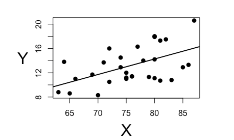
    In the simple linear regression example above, the x-axis represents the selected features (e.g., points, rebounds, or field goal percentage), while the y-axis represents the probability of winning [19]. Each data point represents a team rank based on the selected features. This determines how closely they fit the trend of sinning games.

Gaussian Naïve Bayes

    Gaussian Naïve Bayes (GNB) is a probabilistic classification model built on Bayes’ Theorem. Bayes’s Theorem updates the probability of something happening based on evidence. It uses prior knowledge to determine how likely something is to happen based on this evidence. This is applied to different scenarios, such as how likely one team is to win against several other teams using the data set [23].This model assumes that all the features are independent of each other. This means that the model does not assume that there is any relationship between two features that lead to the predicted outcome; rather, they each impact the prediction in their own way. This assumption allows for simpler computation of the probabilities. This also makes this model very efficient for large data sets[27].

    The Gaussian variant of Naïve Bayes assumes that the features follow a normal distribution. This allows for ease of use for data that is continuous, where the data and its features follow a more bell-shaped curve. For prediction, NBA game features could include points scored, assists, or rebounds, which often follow a normal distribution over large data sets. Also, GNB supports both binary and multiclass classification, which makes it adaptable to predicting various game outcomes.

    Although GNB is simple, the model’s assumption that all features are independent of each other could limit its performance when the features have a strong correlation, such as assists and field goals, since these two go hand in hand in a game. The efficiency of the model allows for a powerful model that is a step up from a linear regression.

Random Forest Classifier

    A random forest classification is a combination of learning methods that build several decision trees and combine all of their predictions to improve accuracy and limit overfitting [27]. This classifier uses parallel ensembling rather than a single equation like linear regressions do. Parallel ensembling trains multiple decision trees separately using different subsets of data and collecting their results through averaging.

\[ G(E) = 1 - \sum_{i=1}^{c} p_i^2 \]

    The above equation is the mathematical formula for the random forest classifier. Gini Impurity G(E) used for decision tree splits in Random Forest. Where p_i is the probability of class i occurring in a particular node, and c is the number of classes [27]. This function assesses the likelihood of selecting an incorrect classifying element. Random forest classifiers are useful when handling larger data sets such as the one used in this tool. An additional use for this model is feature importance. It can help identify the most important factors in determining whether a team will win or lose a game.

Random Forest Classifier Trees

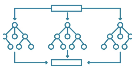
    In the example model, the random forest classifier takes in the large data set and generates multiple decision trees. Each decision tree makes a prediction by looking at different features at each point where the model branches[4]. For instance, one tree may prioritize points scored, while another branch may consider more defensive rebounds a better indicator of a team winning. The final classification is determined by voting across all of the decision trees.

XGBoost

    Extreme Gradient Boosting (XGBoost) is an advanced tree-based learning method that builds a sequence of decision trees where each of the subsequent trees attempts to fix the errors of the previous tree. The optimization function of XGBoost consists of two main components. A loss function measures the performance of the model, while a regularization term penalizes complexity to prevent overfitting. A loss function aims to measure the difference between a model’s predicted output and the actual values that it is trying to predict. This almost acts like an error in prediction. [27].

\[ Obj = \sum_{i=1}^{n} l(y_i, \hat{y}_i) + \sum_{k=1}^{K} \Omega(f_k)\]

    Where l(y_i, ŷ_i) is the loss function that measures the difference between the actual (y_i) and predicted (ŷ_i) values, and Ω(f_k) = γT + (1/2)λ||w||² Regularization is the term to reduce overfitting. The regularization helps limit the model’s complexity by limiting the number of branches and the weight they have on the predicted outcome [27]. When the model trains too well on the provided data, overfitting occurs. This results in very specific patterns that may not align with the general pattern of the data [34].T represents the number of leaves in a tree, while γ and λ are regularization parameters that control the complexity of the model [27].

\[ \hat{y}_i^{(t)} = \hat{y}_i^{(t-1)} + \eta f_t(x_i)\]

    Each prediction is updated iteratively using the above equation. η is the learning rate, which controls how much the models will adjust and update to improve their accuracy. The learning rate takes steps in updating the predictions. A higher learning rate will take larger steps and have faster learning [brownlee_2020?]. f_t is the added decision tree at iteration t [27].

Support Vector Machine

    Support Vector Machine (SVM) is a supervised learning algorithm that constructs a hyperplane or a set of hyperplanes to separate different classes of data in a high-dimensional space. An example of classes being separated based on a set of hyperplanes is shown below [8]. The goal is to find the hyperplane with the largest difference between the two classes. The strength of SVM is its ability to handle both linear and non-linear classification with kernel functions. The kernels map out input data to the higher dimensions to handle relationships [27].

Support Vector Machine Graph

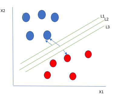
    SVM looks to limit the generalization error by finding the maximum space between classes. This is effective when dealing with overfitting since it makes the model effective in the classification of data. Its ability to handle linear and non-linear datasets makes it a strong model for predicting NBA games, especially when dealing with complex fields that interact with one another to find the predicted winner of a game.

Flask

    In addition to all of the machine learning algorithms and data collection, there is a Flask dashboard that is coded in Python that displays all of today’s NBA games and each model’s predicted winner. Flask is a Python-supported library that makes it easy to create a dashboard or website with HTML and Python code [26]. The website will allow users to simply look at the predictions rather than sorting through complex code and analytics.

Front End

    The dashboard itself is straightforward to avoid any confusion with what the user is looking at. It is set up in a table format with a heading for the start time, home team, away team, and a header for each of the machine learning algorithm’s predictions. In addition to the text of the home and away teams, the team’s logo is displayed for easy readability. This scenario is also the case for each of the predicted winning teams, where the winning team logo is shown with the team name, but the logo is in a green color to indicate that that team is the project winner of that game. The predictions and current games are in a table. The layout allows for easy readability across all columns and rows. Below is how the table and the predictions for each part of the table are set up.

<table class="table table-striped table-dark">
                <thead>
                    <tr>
                        <th>Home Team</th>
                        <th>Visitor Team</th>
                        <th>Start Time (ET)</th>
                        <th>Linear Prediction</th>
                        <th>XGB Prediction</th>
                        <th>Random Forest Prediction</th>
                        <th>Support Vector Prediction</th>
                        <th>Gaussian Naive Bayes Prediction</th>
                    </tr>
                </thead>

    This segment of code sets up the table that displays on the Flask app. The class specifies the type of table in use. There is no specific name for the table head, so it goes right into the header for each of the columns. The home team, visitor team, and start time are all gotten from the api. The other columns of the table are gotten from the predicted winners based on each methods.

{% for game in games %}
  <tr>
    <td>
      <img src="{{ url_for('static', filename='nbalogos/' 
      + game['Home/Neutral'] + '.png') }}" 
        alt="{{ game['Home/Neutral'] }} logo" class="team-logo">
         {{ game['Home/Neutral'] }}
          </td>
            <td>
              <img src="{{ url_for('static', filename='nbalogos/' 
              + game['Visitor/Neutral'] + '.png') }}" 
                alt="{{ game['Visitor/Neutral'] }} logo" 
                class="team-logo">
                {{ game['Visitor/Neutral'] }}
                </td>
                  <td>{{ game['Start (ET)'] }}</td>

{% if game['Linear Prediction'] %}
  {{ game['Linear Prediction'] }}
     <img src="{{ url_for('static', filename='nbalogos/' 
     + game['Linear Prediction'] + '.png') }}" 
      alt="{{ game['Linear Prediction'] }} logo" 
      class="prediction-logo">

    On the Flask dashboard, the NBA logo for the designated team is shown. The code above demonstrates this process. Each of the team’s logos is located in a static folder. The path of the folder is designated with the img src variable. To get the specific team’s logo, the team name from the api is used. This name also matches the .png file; for example, the Cleveland Cavaliers appear as Cavaliers in the API, and the PNG is Cavalier.png. This is done for the home and away team columns as well as each model’s columns. The images in the model’s prediction columns appear green. On the Flask dashboard, the NBA logo for the designated team is shown. The above code shows how this task is done. Each of the team’s logos is located in a static folder. The img src variable designates the folder’s path. To get the specific team’s logo, the team name from the api is used. This name also matches the .png file; for example, the Cleveland Cavaliers appear as Cavaliers in the nba_api, and the png is Cavalier.png. This procedure is done for the home and away team columns as well as each model’s columns. The images in the models’ prediction columns appear green.

    An additional small feature on the dashboard is the implementation of the current time. Above the table, the data and current time the user is accessing the dashboard are displayed so they can see when a particular NBA game starts relative to the current time. Along with the current time, the text is displayed, letting the user know that games update at 12 p.m. Eastern time every day and that there is a game. This is due to how the API gets live games for the day. The overall color scheme is a black background with a grey table. Each of the texts on the page is white for easy readability. The table also has green accents on it, the predicted team logos are green, allowing for high contrasts between the green and the darker backgrounds.

Back End Integration

    The most important part of this tool is the model outputs generated by each predictive mode. Each of the models has a separate folder where the machine learning process takes place and the model’s file is put. The above function has to be called by the backend of the Flask dashboard. In most cases, the outputted file will either be a JSON or a .pkl file. The execution of each of the models to output their .pkl or JSON is as follows. The linear regression model took 0.04 seconds to output its prediction file, while the Gaussian Naive Bayes (GNB) algorithm took 0.07 seconds. The support vector machine took the longest time to run, with an execution time of 32.18 seconds. In the middle of the pack, the Random Forest classifier took 18.14 seconds to complete, and XGBoost took a total time of 12.69 seconds. These two file types allow for the machine learning model’s algorithm and predictions to be called in the Flask app. JSON files are text-based and contain data that is readable by machines and humans. Only XGBoost uses JSON files in specific cases that require special configuration [1]. Here is an example of the linear regression model called into the dashboard

linear_model =joblib.load('models/linear-regression/linear_model.pkl')

The first function that is in the Flask app is called predict winner. Here is the header of the function.

def predict_winner(home_team, away_team, model_type='linear')

    Within this function, several variables need to be defined. First, the data set that the models were trained on needs to be pulled. Then the features that the models are trained on need to be defined. In the case of the base, these features are eFG%, OREB%, TOV%, FTr, and DREB%. Each team’s stats then need to be assigned a variable based on their name and whether they are the home or away team. That information is then put into a data frame for predictions. The final input of the predicted_winner function is what model is used The default is linear, but each model has its own string to allow for the designated model to produce a prediction. Below is how each model is defined.

comparison_data = pd.DataFrame([team_home_stats, team_away_stats], 
  index=[home_team, away_team])

if model_type == 'linear':
        predicted_ranks = linear_model.predict(comparison_data)
    elif model_type == 'rf':
        predicted_ranks = rf_model.predict(comparison_data)  
    elif model_type == 'svm':
        predicted_ranks = svm_model.predict(comparison_data)
    elif model_type == 'nb':
        predicted_ranks = nb_model.predict(comparison_data)
    elif model_type == 'xgb':
        dmatrix = xgb.DMatrix(comparison_data)
        predicted_ranks = xgb_model.predict(dmatrix)
    else:
        return None

    This large if else statement gets the data frame for each of the models to store their prediction. It takes in both the away and the home teams’ stats and creates a data frame. The machine learning model is chosen based on the ‘model_type’. It then uses the chosen model’s prediction for both teams to find a winner.

    The second function in the Flask application is to fetch the live games for the day as well as call the predicted_winner function. Using the nba_api each game is gotten for the day and each away and home team is assigned a variable to allow for them to be inputted into the predicted_winner function. Each game is predicted by each model and then added back to a previously defined list. This list is what allows for the HTML to display the predictions and other necessary information for each game.

if game_time_ltz.date() == today:
  away_team = game['awayTeam']['teamName']
  home_team = game['homeTeam']['teamName']

  # Get predictions from models
  linear_prediction = predict_winner(home_team, away_team, \
                                  model_type='linear')
  xgb_prediction = predict_winner(home_team, away_team, \
                               model_type='xgb')
  rf_prediction = predict_winner(home_team, away_team, \
                              model_type='rf')
  svm_prediction = predict_winner(home_team, away_team, \
                               model_type='svm')
  nb_prediction = predict_winner(home_team, away_team, \
                              model_type='nb')

    The first part of this code section checks is the game that is being predicted is scheduled for that day. It then gets each of the home team and away team’s names. The five different machine learning models are then used to predict the winner between the two teams that were gathered. The predict winner function is used to do this. Each prediction is stored in its own variable to be called later.

# Add the game details and predictions to the list
  todays_games.append({
    'Game Date': game_time_ltz.strftime('%Y-%m-%d'),
    'Start (ET)': game_time_ltz.strftime('%I:%M %p'),
    'Visitor/Neutral': away_team,
    'Home/Neutral': home_team,
    'Linear Prediction': linear_prediction,
    'XGB Prediction': xgb_prediction,
    'Random Forest Prediction': rf_prediction,
    'Support Vector Prediction': svm_prediction,
    'Gaussian Naive Bayes Prediction': nb_prediction
    })

    The above code snippet sets up the dictionary that is then used in the HTML to display the games and the predicted winner of the day’s NBA games.

Conclusion of Methods

    This section of methods outlines the key steps that were taken in the development of the tool to predict the outcomes of NBA games. Included in these steps are model selection, feature selection, and integration with a Flask dashboard. Using the five models that are in the section above, the tool establishes a framework for predicting games with the predictive machine learning models. These models were selected based on their high ability in sports prediction and ability to find trends in large data sets.

    The integration of these models with a Flask-based dashboard allows for ease of use for users and allows for simple readability. The steps taken in the back end of the tool allow for each day’s NBA games to be shown as well as the prediction for each of these games.

    Having a baseline model with the initial setup allows the tool to take the next step in evaluating its effectiveness and accuracy. The next section is all about experimenting with settings in the models used in the tool. Adjusting the data test split and features for each model will allow for testing of accuracy with different variables. Assessing the reliability of the tool will be done by comparing predictions from the tool and comparing them to real-world NBA game outcomes.

Experiments

Baseline

    As previously mentioned, the features used as a baseline for experiments are from Dean Oliver’s “Four Factors of Basketball Success.” The features used are Effective Field Goal Percentage (eFG%), Offensive Rebound Percentage (OREB%), Turnover Percentage (TOV%), Free Throw Rate (FTr), and Defensive Rebound Percentage (DREB%). The data set of NBA games for each of the previously mentioned five models is split into an 80% training set and a 20% test set. Each model’s predictive accuracy has been recorded at these baselines based on a percentage from the predicted winners compared to the actual winner of the NBA games.

    It is also important to note that all of these experiments and tests have been done on an Apple M3 chip with 16GB RAM. Run and compiling times for each of the models may vary based on the machine used to run them.

Data Split Experiment

    The first experiment tests how changing the data designated for training and testing sets affects the performance of the model. The baseline configuration uses 80% of the data for training and 20% for testing. For this experiment, the training set is adjusted to 70%, and the testing set is increased to 30%. The goal is to see how the predictions change based on the portions affected. This will be done by comparing each of the models against each other for the accuracy of prediction.

Best Features

    This experiment explores the effect of modifying the features used by each mode. A random forest classifier model is used to determine feature importance. The classifier ranks each of the features in the data set based on how likely they are to impact the target, which in this case is a team winning. Based on the result of the classifier, the top five features were selected. Below are all of the rankings of the features in the data set. Each model will be assessed using the baseline features and the best features from the random first classifier. Both will have their accuracy recorded to compare precision.

List of features and their importance to predicting winners

Feature	Importance
ORTG	0.1158
DREB	0.0964
eFG%	0.0867
REB	0.0751
TS%	0.0660
PTS	0.0504
FG_PCT	0.0471
STL	0.0394
FG3_PCT	0.0349
POSS	0.0324
TOV%	0.0255
FGM	0.0245
DREB%	0.0242
OREB%	0.0221
PF	0.0221
FT/FGA	0.0213
FTr	0.0209
FT_PCT	0.0209
BLK	0.0203
AST%	0.0202
AST	0.0197
FG3A	0.0185
TOV	0.0175
FGA	0.0174
FTA	0.0161
FTM	0.0159
OREB	0.0145
FG3M	0.0143
REB%	0.0000

Cross Validation

    The final experiment is cross-validation, which is used to provide a more in-depth evaluation of each model’s performance. This is done by splitting the data into multiple sets and testing the model on each of them. This method allows for a more generalized assessment of the model’s ability to predict NBA game outcomes. The performance of the cross-validation experiment is compared across the baseline, data split, and best feature selection experiments. Evaluating the result from each of the models can help assess the impact of different strategies on the prediction accuracy for each model.

Model Accuracy

    This section incorporates the baseline, changed test data split, and best features model. This will be compared for real-world accuracy based on their predicted results of around 50 NBA games and each of these games’ real winners. In addition to the accuracy of the tool and real-world outcome, various metrics were used to evaluate each of the model’s performances. These metrics were used from the scikit-learn library, and they include precision, recall, F1 score, ROC AUC, and R². The precision quantifies the number of correct predictions among the positive cases, such as an NBA team winning. In return, this limits false positives. Recall looks at the ability of the model to identify the positive cases; this will let us know how well the models find the correct winner of the game [9]. The F1 score is a mean of the precision and the recall; this allows for a balance in finding how often the models will predict the correct outcome. ROC AUC (Receiver Operating Characteristic - Area Under Curve) measures how well the models can determine the winners and losers of an NBA game. The higher the ROC AUC value is, the better it is at making the distinction between winners and losers. Finally, R² is the coefficient of determination that looks at the variance in the target variable, which is winning. Positive values of R² suggest that the model has a high predictive value [7].

Baseline Real-Life Accuracy Comparison

Baseline Model Evaluation

Model	Accuracy	Precision	Recall	F1-Score	ROC AUC	R2
LR	56.14%	0.71	0.72	0.71	0.78	0.23
XGB	47.37%	0.72	0.73	0.72	0.72	-0.10
RF	54.39%	0.70	0.71	0.70	0.70	-0.18
SVM	59.65%	0.72	0.72	0.72	0.72	-0.12
GNB	59.65%	0.70	0.69	0.70	0.69	-0.20

    The table above shows the accuracy of each model when using the baseline. The highest accuracy models are SVM and GaussianNB, with nearly a 60% accuracy when predicting real-life games. Linear regression and Random Forest classifiers’ accuracy were slightly below the top with around 55% accuracy. Most interestingly, XGB was the lowest-performing model. Traditionally, we would think that the linear regression model would be the lowest performing due to it not being complicated and not analyzing and finding relationships in the data; rather, it is a linear plane that fits and ranks teams. The low performance of XGB might suggest that it is overfitting the data that is being used.

    Beyond the real-life accuracy of the models, linear regression shows the strongest overall performance when compared to the other models and their various metrics. With an ROC AUC of 0.78, linear regression has the highest ability to distinguish between a team winning and losing. XGBoost and random forest struggle with lower accuracy, ROC AUC, and negative R² scores. This suggests that there are some limitations with the predictions of NBA games for these models. This is due to their lack of ability to differentiate between winning and losing teams.

Real-life Accuracy Results with 30% Test Data

70/30 Train Test Split Model Evaluation

Model	Accuracy	Precision	Recall	F1-Score	ROC AUC	R2
LR	54.39%	0.73	0.71	0.72	0.79	0.25
XGB	45.61%	0.73	0.72	0.73	0.72	-0.10
RF	50.88%	0.71	0.70	0.71	0.71	-0.17
SVM	57.89%	0.72	0.71	0.72	0.72	-0.13
GNB	57.89%	0.69	0.69	0.69	0.69	-0.24

    Using a 70/30 training test split again, SVM and GaussianNB achieved the highest accuracy at predicting real-world games at nearly 58% accuracy. In this experiment, linear regression was better, with a 54% accuracy, than random and XGB. As seen in the baseline, XGB is still struggling to have high accuracy when predicting the correct outcomes of the game, suggesting the model is still possibly overfitting and struggling with the real-world use of the data that it is given. The changing of the training test split has lowered the accuracy of the models between 2% and 4%. This finding suggests that higher testing sets could lower the accuracy of predicting NBA game outcomes.

    Once again, in this experiment, linear regression stands out as having the best overall balance across all metrics. The model still has the highest ROC AUC at 0.79 and has an F1 score that is pretty similar to the rest of the models. XGBoost and random forest are still underperforming with a test-training split experiment. Both of these models have low accuracy and negative R² values. This evidence suggests that the models are still struggling to find patterns in the data that are meaningful for predicting NBA game outcomes. With four of the five models having negative R² scores, it is important to consider that the models may be having issues with feature selection and optimization issues beyond the test-training set split in this experiment.

Real-Life Accuracy Using the Best Features

Best Features Model Evaluation

Model	Accuracy	Precision	Recall	F1-Score	ROC AUC	R2
LR	52.63%	0.81	0.82	0.82	0.90	0.22
XGB	50.88%	0.82	0.80	0.81	0.81	0.25
RF	66.67%	0.81	0.80	0.80	0.81	0.23
SVM	57.89%	0.81	0.82	0.82	0.82	0.27
GNB	57.89%	0.81	0.80	0.80	0.81	0.22

    Using the five best features from feature importance, Random Forest saw a large increase in accuracy with a 66.67% accuracy in real-world game prediction, which is the best by nearly 10% in this experiment. The SVM and GaussianNB models achieved an accuracy of 57.89%. It is intriguing and important to note that these two models’ accuracy still lowered from the baseline but still had the same accuracy as the experiment where the training test split was modified. The accuracy of linear regression slightly decreased from the baseline, reaching 52% accuracy. XGB saw an increase in accuracy in this experiment at the baseline. With a 50.88% accuracy, it has jumped about 5% from the baseline and the training test split experiment. Furthermore, XGB is keeping the trend of struggling with predicting real-world outcomes. Taking everything into account, the case emphasizes the importance of choosing the right features when creating predictive models.

    Aside from the models having higher real-world accuracy, the five best features also boosted performance across all the models. Even though random forest had the highest overall accuracy, linear regression, SVM, and XGBoost had strong metrics and notable increases. SVM and linear regression performed well for F1-scores, suggesting that they are well-rounded when it comes to classification performance. A surprising metric that came from testing the model was linear regression achieving a 0.90 when it comes to ROC AUC, which tells us that it does well separating winners and losers. A notable metric that changed with the best feature is the R² scores. None of the scores are negative, showing that each of the models is capable of finding variance in the data.

Cross-Validation Results

Base-line Cross-Validation Results

    A cross-validation experiment with five folds was done to evaluate the performance of each of the five models when predicting NBA game outcomes. This experiment was done on the baseline models, the models where the test size was changed to 30%, and the models where the best features from feature importance were used. The tables in this section contain accuracy scores from each fold as well as the average accuracy.

Baseline Model Cross-Validation

Model	Fold 1	Fold 2	Fold 3	Fold 4	Fold 5	Mean Acc.
LinReg	0.2634	0.2463	0.2520	0.2521	0.2681	0.2564
XGB	0.7221	0.7249	0.7151	0.7297	0.7406	0.7269
RF	0.7036	0.7020	0.6949	0.7058	0.7162	0.7045
SVM	0.7189	0.7085	0.7123	0.7265	0.7200	0.7172
GNB	0.7064	0.6911	0.6960	0.6841	0.6987	0.6953

    The table above shows the results from the baseline tool. These results indicate that XGBoost (XGB) had the overall highest average accuracy at 0.7269 and the overall highest fold in fold 5, where the accuracy was 0.7406. SVM was very similar to XGB with an average accuracy of 0.7172, and similarly, Random Forest had an average accuracy of 0.7045. Gaussian Naïve Bayes takes a slight dip in accuracy at 0.6953 when compared to the best performer of XGB. The linear regression has the worst average accuracy out of the group at 0.2564. The linear regression models suggest that taking a linear approach to predicting NBA games is not sufficient since it does not take into account all the complex relationships between the data sets. Tree-based methods such as XGB and random forests, as well as kernel-based methods such as SVM, perform much better. Overall, each model was rather consistent in each fold for accuracy. XGB shows high accuracy, suggesting that it is effective for predicting NBA games.

Cross-Validation Results with 30% Test Data

    The table below displays the cross-validation results for the models with a test data split of 30% instead of 20%. The accuracy scores for each fold as well as the average accuracy across each of the five folds for every model.

70/30 Training Test Split Model Cross-Validation

Model	Fold 1	Fold 2	Fold 3	Fold 4	Fold 5	Mean Acc.
LinReg	0.2605	0.2468	0.2489	0.2477	0.2743	0.2552
XGB	0.7203	0.7197	0.7234	0.7265	0.7520	0.7284
RF	0.7067	0.7110	0.7023	0.7060	0.7209	0.7098
SVM	0.7178	0.7110	0.7141	0.7247	0.7253	0.7190
GNB	0.6861	0.6917	0.6967	0.7122	0.7048	0.6987

    Changing the test split slightly impacted the performance of some of the models. XGBoost still was the best-performing model with an average accuracy of 0.7284 and again had the highest accuracy fold in fold five with an accuracy of 0.7520. SVM and random forest still remain less accurate but get a slight boost in overall accuracy with 0.7190 and 0.7098, respectively. It is intriguing to note that Gaussian Naïve Bayes performed slightly worse than the baseline. Linear regression remained the weakest model in accuracy across all folds. This experiment shows that affecting the size of the model’s data test split can affect accuracy across cross-validation experiments. It also shows that tree-based and kernel-based methods still outperform simpler linear models.

Cross-Validation Results with Best Feature Selection

    In this table, the models used features based on feature importance rankings. Below are the accuracy scores for each fold and the average accuracy across five folds for each model.

Best Features Model Cross-Validation

Model	Fold 1	Fold 2	Fold 3	Fold 4	Fold 5	Mean Acc.
LinReg	0.4344	0.4331	0.4436	0.4451	0.4419	0.4400
XGB	0.8070	0.8102	0.8282	0.8146	0.8167	0.8153
RF	0.8037	0.7852	0.8026	0.8010	0.8010	0.7987
SVM	0.8140	0.8059	0.8249	0.8167	0.8151	0.8153
GNB	0.7972	0.7868	0.8004	0.7874	0.7776	0.7891

    Selecting the top five most important features improved model preference and accuracy across the board. XGB and SVM had the highest average accuracy at 0.8153. This result is roughly a .1 jump from the baseline, showing the effectiveness of selecting the right features to improve predictive accuracy. Random forest had an average accuracy of 0.7987, while Gaussian Naïve Bayes had an average accuracy of 0.7891. Both of these models had a decent jump in accuracy. The biggest jump in accuracy was from linear regression. In the baseline cross-validation, linear regression had an average accuracy of 0.2564, while the linear model in this experiment jumped to an average accuracy of 0.44. With this being said, it still underperforms when compared to the other four models. This experiment shows the importance of features when it comes to model efficiency and accuracy.

Threats to Validity

    One threat to validity in these experiments is the splitting of data into test and training sets. As seen in the experiment where the training set to test set ratio was split into 70:30, it changed how well the predictions were made compared to the baseline model, which had an 80:20 training set to test set ratio. Different splits can lead to different performances in accuracy from different models, which can lead to potentially inaccurate evaluations of how well the models perform.

    Another important concern from the experiments is how poorly XGB performed when tested on real-world results. This can be due to overfitting and generalization. When running cross-validation experiments, XGB performed well throughout each of the tests but struggled with its real-world application. The overfitting or generalization can lead to the results of the model being inaccurate compared to what the model’s prediction capabilities are.

    Using a random forest classifier to select the best five features based on feature importance resulted in the biggest performance increase. Such an approach has the possibility of introducing feature bias. Each model may not use and predict outcomes as well as another when using these five features, leading to inaccurate results.

    The data set that was used for all models was from the last five full seasons of NBA games. It is possible that there could be better results using both a smaller dataset and a larger dataset. For instance, using 3 seasons or 10 seasons could help or hurt finding trends in the data for prediction.

    A final threat to the validity of the experiments and the tool’s accuracy is the lack of contextual factors when predicting NBA games. Having a team have a slight advantage when playing at home could increase the accuracy of the models. The biggest contextual factor that is missing is how and what player affects the team’s stats. From season to season, teams change in small and large amounts that can impact the team’s overall performance. The biggest example of this that was shown in this model when recording accuracy was when a large trade was done in season. The Dallas Mavericks have better stats due to their star player. The player on the Mavericks was then traded, which affected their team as a whole. So when the model predicted games for the Mavericks, it would often have them as the predicted winner because they were a much better team prior to this trade.

Conclusion

Summary of Results

    The goal of this project and thesis was to achieve the highest accuracy possible in predicting NBA games using machine learning and predictive algorithms. By using historical data from the past 5 years of the NBA that was obtained from the nba_api, machine learning algorithms were evaluated for their effectiveness in predicting daily NBA games. The research that was done included examining key features that affect the outcomes of NBA games, such as field goal percentage, rebounds, assists, and points, as well as advanced metrics such as offensive efficiency and effective field goal percentage. Five machine learning models—Linear Regression, Random Forest, XGBoost, Support Vector Machine, and Gaussian Naïve Bayes—were used and tested with the obtained NBA data to assess their effectiveness in predictive outcomes

    Throughout this study, it was clear that the complexity of machine learning plays a large role in the accuracy of NBA game prediction. The more complex algorithms, such as Support Vector Machine and Random Forest, outperformed simpler models like Linear Regression and Gaussian Naïve Bayes. With this being said, the cross-validation experiment results showed high accuracy, but when it came to the real-world application of the models, it was highlighted that there were challenges in translating the model from test accuracy to real-world accuracy. Factors such as overfitting missing contextual data, as well as unpredictable in-game events, could have affected the accuracy of these models when predicting real-world NBA games.

    Changing the train-test split ratios had an apparent impact on prediction. When the baseline’s 80/20 split was changed to a 70/30 split, the model’s accuracy slightly decreased. These results suggest that changing the train-test split ratios can influence performance. This reinforces the need for careful selection of the testing and training ratios. Additionally, using the top five features from feature importance led to significant improvements not just in accuracy but across all of the metrics tested. The Random Forest Classifier had the largest increase in accuracy, but across all models, there was an increase in accuracy. When using the top five features from feature importance, it showed notable improvement in the accuracy of the models. The effect was apparent in the large jump that the Random Forest Classifier had in accuracy. Selecting features that have the highest impact on winning is important for achieving higher accuracy in predictive models. Precision, recall, F1-score, ROC AUC, and R² all had gains with the top five selected features. The change from 4 out of 5 models having a negative R² value shows the importance of selecting features that increase the accuracy of predicting NBA games.

    Despite the promising results, this study shows some key limitations of machine learning models in sports prediction. There are numerous external factors, such as injuries, trades, coaching decisions, and player load management were not accounted for in the models and the tool as a whole. These factors can have a significant impact on NBA game outcomes and these factors will and can change day to day. Based on the research and the results of the testing real-time contextual data could increase the accuracy of the models used. Machine learning provides valuable insight and analytics for predicting NBA games; the accuracy of the models in some cases leaves more to be desired. With limited access to external factors that are not present in the data set they are predicting off of, they may not be as effective as they can be.

    Overall, this study shows that machine learning can be a useful tool for predicting NBA games, but it is difficult to achieve high rates of accuracy over a long period of time. For this to happen, more optimizations would need to be made to the tool. Three levels of success are distinguished. The first are the models that were around 60% accurate. The models that achieved this mark would be considered successful. Being able to predict the outcome of a game with that level of accuracy is consistent enough to be trustworthy. If you think about betting on teams and you win 60% of the time, you are winning a large portion of your bets. The next level of success is somewhat successful. These models are around 55% accurate. The accuracy of the model is greater than a coin flip but not consistent enough to be trusted. Finally, the failures of the models are those that are 50% and below. This is a coin flip. With proper research and looking into NBA teams, you could predict the outcomes of NBA games at the same or a higher rate than these models, which are at or below 50% accuracy. Several additions can be made to the tool to help increase its accuracy and effectiveness. Expanding the dataset, integrating live data, and improving feature selection are the next steps for this tool.

Future Work

Model Enhancement

    This tool can undergo several enhancements to increase its accuracy in predicting NBA game outcomes. Currently, the tool does not have any contextual factors incorporated into predicting the winners of each game. Some contextual factors that could be added to improve the tool are home-court advantage, player rest days, and trades. There would need to be more code written to see how each player has an impact on their team winning. Trades in the season and the offseason would also need to be live data. Trades in between seasons are most important since stats can vary based on who was traded.

    Incorporating home-court advantage would allow for more realistic predictions in the real world. For some teams, it may be evident in the data that they are a better team when they play at home rather than on the road. Incorporation of home court advantage would give these types slightly better odds when predicting the winner. Similarly, factoring in player injuries and rest days could impact the accuracy of the models. This type of analysis would factor in the impact of each player on a team and how they contribute to winning. To do this, external data sources would be needed, like an API, to get day-to-day changes in injury reports and rest days.

    Trades can also affect the performance of a team, whether it is in a season or in between seasons of the NBA. The tool currently does not adjust for any kind of roster changes. This could lead to inaccuracies among the team’s stats due to a player not being on the team anymore. A player who was traded may have had a large impact on that team’s stats for a particular season. Future versions of the tool would want to have a method of tracking roster changes and changing predictions accordingly to these changes.

    Apart from statistical improvements, additional advanced metrics can be incorporated into the tool, such as adjusted plus-minus ratings, player efficiency ratings, and real-time injury reports. These statistics are not a part of the data set because they are not calculated from the data that was already provided by the API. On the user side of the tool, adding sportsbook odds into the dashboard for each game can help the user see all of the model’s predictions and compare them to who the sportsbooks are predicting to win. This feature offers more context to the user on the predicted outcomes.

Machine Learning Enhancements

    This project focused only on five machine learning models, but there are numerous other machine learning algorithms and predictive models that could enhance prediction accuracy or perform better than the models chosen for this tool. Future model implementations should look into deep learning algorithms, such as neural networks. Neural networks can process large amounts of data and find complex patterns better than traditional models. Several forms of neural networks can be useful when predicting NBA games that capture profound relationships within data sets. In addition to neural networks, combining models to make a prediction could be more accurate than each of the models doing this separately. Each model can use their strengths for one combined prediction.

    The current implementation of the tool has the user manually adjust the feature in the Python code. To enhance the tool’s user-friendliness, we propose enabling the user to choose the features they wish to predict games for directly from the dashboard. This approach would allow users to experiment with the features used and how they impact the predictions from the models. Ideally, this could be a drop-down menu where the user selects as many features as they want, and the model would then spit back out the predictions using the newly refined features.

    Finally, the tool only predicts the winner of the games. Future implementation of this tool could predict the point spread, how much a team will win by, or the total number of points scored in an NBA game. This calculator could provide a more complete tool when it comes to predicting all aspects of NBA games.

Data Collection and Live Updates

    As previously mentioned, a static CSV file stores all the current data. This restriction limits the tool’s ability to use the ever-changing stats during the current NBA season. To make the system more dynamic, use web scraping or APIs to get live game stats and save them for future predictions. Using real-time data collection, the tool would always be updating the model’s data sets and have the most up-to-date stats for prediction.

    Implementing live data would allow for the models to be more adaptive when predicting NBA games. The live data would include many stats that were not previously in the CSV files. This data would show how a current team is doing in the season rather than just in the past season.

Future Ethical Implications

    One of the main ethical concerns with predictive modeling is the potential for bias. The models are trained on past NBA data, which could present a risk in historical biases that may influence the prediction from the tool. For instance, the model may favor teams that have historically performed very well but now do not account for large changes in roster from the past season to the current season. To limit this bias, there needs to be ongoing analysis to make sure that the models are fair and are unbiased, especially when teams go from season to season and have blockbuster trades.

    Being transparent is also an important aspect of the development process. Users need to clearly understand how models make their predictions as well as what features are used. Furthermore, the user should be made aware of the potential impacts that each of the features selected can have. Providing users with explanations of what each decision is with each model as well as how they work is important to limit confusion.

Sports Betting and Gambling

    This tool is intended for analytical and informational uses, but there is always a possibility that users may leverage the information from the tool for sports betting. Predictive models can influence betting behavior, which is irresponsible gambling if the user blindly trusts each of the models and how accurate they are.

    To limit this risk, there are disclaimers included in the tool’s documentation and interface to make sure that the user should not trust each of these predictions as if they were accurate 100% of the time. Educating the user about uncertainties in sports prediction can help make sure they are not overly reliant on this tool and use some of their research and thoughts.

Closing thoughts

    This thesis and the tool that goes along with it show the potential of machine learning algorithms’ predictive abilities when used on NBA games while also showing the complexities of achieving a high accuracy result from them. Even though there are significant findings in the experiments that were run, there is still more that can be done to make the predictive accuracy better. Contextual factors can add another layer of predictive ability to the models and have the potential to improve accuracy.

    Using machine learning in sports prediction still has its challenges, but there are endless possibilities in how machine learning models can be used to create tools that predict not just NBA games and their stats but all of the other sports in the world. This tool is a step in the direction of the world of predictive analytics that is ever-growing.

References

[1]

Apple. Pkl. Retrieved from https://pkl-lang.org/

[2]

Rory P. Bunker and Fadi Thabtah. 2019. A machine learning framework for sport result prediction. Applied Computing and Informatics 15, 1 (2019), 27–33. https://doi.org/https://doi.org/10.1016/j.aci.2017.09.005

[3]

Hayden D Cahill, Ross Gordon, Lauren Gurrieri, and Theresa Harada. 2024. How platformisation shapes sports betting consumption practices and implications for harm. Marketing Theory (2024), 14705931241270853.

[4]

Mohit Chaudhary. 2025. Random forest algorithm - how it works & why it’s so effective. Retrieved from https://www.turing.com/kb/random-forest-algorithm

[5]

Dimitrije Curcic. 2023. NBA popularity stats. (2023).

[6]

eMarketer. 2024. Number of monthly live sports viewers in the united states from 2022 to 2027, by platform type. (2024).

[7]

GeeksforGeeks. 2024. Metrics for machine learning model. Retrieved from https://www.geeksforgeeks.org/metrics-for-machine-learning-model/

[8]

GeeksforGeeks. 2025. Support vector machine (SVM) algorithm. Retrieved from https://www.geeksforgeeks.org/support-vector-machine-algorithm/

[9]

Google. 2025. Machine learning crash course: Classification: Accuracy, recall, precision, and related metrics. Retrieved from https://developers.google.com/machine-learning/crash-course/classification/accuracy-precision-recall

[10]

Tomislav Horvat and Josip Job. 2019. Importance of the training dataset length in basketball game outcome prediction by using naive classification machine learning methods. Elektrotehniški vestnik 86, 4 (2019), 197–202.

[11]

Tomislav Horvat, Josip Job, Robert Logozar, and Časlav Livada. 2023. A data-driven machine learning algorithm for predicting the outcomes of NBA games. Symmetry 15, 4 (2023). Retrieved from https://www.mdpi.com/2073-8994/15/4/798

[12]

Matthew Houde. 2021. Predicting the outcome of NBA games. (April 2021).

[13]

Jiayi Lu, Yuan Chen, and Yida Zhu. 2019. Prediction of future NBA games’ point difference: A statistical modeling approach. In 2019 international conference on machine learning, big data and business intelligence (MLBDBI), 2019. IEEE, 252–256.

[14]

Batta Mahesh. 2020. Machine learning algorithms-a review. International Journal of Science and Research (IJSR).[Internet] 9, 1 (2020), 381–386.

[15]

Carolyn Mair, Gada Kadoda, Martin Lefley, and Keith. 2000. An investigation of machine learning based prediction systems. Journal of Systems and Software 53, 1 (2000), 23–29. https://doi.org/https://doi.org/10.1016/S0164-1212(00)00005-4

[16]

Carolyn Mair, Gada Kadoda, Martin Lefley, Keith Phalp, Chris Schofield, Martin Shepperd, and Steve Webster. 2000. An investigation of machine learning based prediction systems. Journal of systems and software 53, 1 (2000), 23–29.

[17]

Richard Einstein Doss Marveldoss. 2018. An elo-based approach to model team players and predict the outcome of games. PhD thesis.

[18]

Michael Mondello and Christopher Kamke. 2014. The introduction and application of sports analytics in professional sport organizations. Journal of Applied Sport Management 6, 2 (2014), 11–30.

[19]

Luka Negoita. 2021. How to do a simple linear regression in r | r (for ecology). Retrieved from https://www.rforecology.com/post/how-to-do-simple-linear-regression-in-r/

[20]

Nguyen Hoang Nguyen, Duy Thien An Nguyen, Bingkun Ma, and Jiang Hu. 2022. The application of machine learning and deep learning in sport: Predicting NBA players’ performance and popularity. Journal of Information and Telecommunication 6, 2 (2022), 217–235.

[21]

Shedrack Onwusinkwue Ogugua Chimezie Obi Samuel Onimisi Dawodu and Aske Plaat. 2024. Data science in sports analytics: A review of performance optimization and fan engagement. World Journal of Advanced Research and Reviews (2024), 8.

[22]

Kevin Ota. 2024. ESPN men’s fantasy basketball: 2 million players, 2 years in a row. ESPN Press Room (2024).

[23]

Stanford Encyclopedia of Philosophy. 2003. Bayes’ theorem. Retrieved from https://seop.illc.uva.nl/entries/bayes-theorem/

[24]

Samuele Lo Piano. 2020. Ethical principles in machine learning and artificial intelligence: Cases from the field and possible ways forward. Humanities and Social Sciences Communications 7, 1 (June 2020), 9.

[25]

Sebastian Raschka. 2018. Model evaluation, model selection, and algorithm selection in machine learning. arXiv preprint arXiv:1811.12808 (2018).

[26]

Armin Ronacher and Pallets Projects. 2010. Flask. Retrieved from https://flask.palletsprojects.com/

[27]

Iqbal H. Sarker. 2021. Machine learning: Algorithms, real-world applications and research directions. SN Computer Science 2, 160 (2021). https://doi.org/10.1007/s42979-021-00592-x

[28]

Vangelis Sarlis and Christos Tjortjis. 2020. Sports analytics — evaluation of basketball players and team performance. Information Systems 93, (2020), 101562. https://doi.org/https://doi.org/10.1016/j.is.2020.101562

[29]

Sports Media Watch. 2024. Average TV viewers of the NBA regular season from 2019/20 to 2023/24. (2024).

[30]

Swar. 2025. Nba_api. Retrieved from https://github.com/swar/nba_api

[31]

Siu-Ming Tam and Jae-Kwang Kim. 2018. Big data ethics and selection-bias: An official statistician’s perspective. Statistical Journal of the IAOS 34, 4 (2018), 577–588.

[32]

Fadi Thabtah, Li Zhang, and Neda Abdelhamid. 2019. NBA game result prediction using feature analysis and machine learning. Annals of Data Science 6, 1 (2019), 103–116.

[33]

Meysam Vakili, Mohammad Ghamsari, and Masoumeh Rezaei. 2020. Performance analysis and comparison of machine and deep learning algorithms for IoT data classification. IEEE Access 8, (January 2020), 1699–1712. https://doi.org/10.1109/ACCESS.2020.2965169

[34]

Xue Ying. 2019. An overview of overfitting and its solutions. Journal of Physics: Conference Series 1168, 2 (2019), 022022. https://doi.org/10.1088/1742-6596/1168/2/022022

[35]

Yasi Zhang, Sicheng Zhou, Xi Zheng, Yuyu Wang, and Minrui Liang. 2021. Modeling and predicting the outcomes of NBA basketball games. In Proceedings of the 2021 european symposium on software engineering, 2021. 94–99.